국내프로야구연봉예측
in Study on datavisualization
국내 프로야구 연봉 예측
# 회귀분석으로 미래 연봉 예측
#2017년 연봉, 성적을 가지고 2018년에 연봉 예측

# -*- coding: utf-8 -*-

%matplotlib inline

import pandas as pd
import numpy as np
import matplotlib.pyplot as plt

import warnings
warnings.filterwarnings("ignore")
# 프로야구 연봉 데이터셋의 기본 정보

# Data Source : http://www.statiz.co.kr/

picher_file_path = 'data/picher_stats_2017.csv'
batter_file_path = 'data/batter_stats_2017.csv'
picher = pd.read_csv(picher_file_path)
batter = pd.read_csv(batter_file_path)
picher.columns
Index(['선수명', '팀명', '승', '패', '세', '홀드', '블론', '경기', '선발', '이닝', '삼진/9',
       '볼넷/9', '홈런/9', 'BABIP', 'LOB%', 'ERA', 'RA9-WAR', 'FIP', 'kFIP', 'WAR',
       '연봉(2018)', '연봉(2017)'],
      dtype='object')
picher.head()
| 선수명 | 팀명 | 승 | 패 | 세 | 홀드 | 블론 | 경기 | 선발 | 이닝 | ... | 홈런/9 | BABIP | LOB% | ERA | RA9-WAR | FIP | kFIP | WAR | 연봉(2018) | 연봉(2017) | |
|---|---|---|---|---|---|---|---|---|---|---|---|---|---|---|---|---|---|---|---|---|---|
| 0 | 켈리 | SK | 16 | 7 | 0 | 0 | 0 | 30 | 30 | 190.0 | ... | 0.76 | 0.342 | 73.7 | 3.60 | 6.91 | 3.69 | 3.44 | 6.62 | 140000 | 85000 |
| 1 | 소사 | LG | 11 | 11 | 1 | 0 | 0 | 30 | 29 | 185.1 | ... | 0.53 | 0.319 | 67.1 | 3.88 | 6.80 | 3.52 | 3.41 | 6.08 | 120000 | 50000 |
| 2 | 양현종 | KIA | 20 | 6 | 0 | 0 | 0 | 31 | 31 | 193.1 | ... | 0.79 | 0.332 | 72.1 | 3.44 | 6.54 | 3.94 | 3.82 | 5.64 | 230000 | 150000 |
| 3 | 차우찬 | LG | 10 | 7 | 0 | 0 | 0 | 28 | 28 | 175.2 | ... | 1.02 | 0.298 | 75.0 | 3.43 | 6.11 | 4.20 | 4.03 | 4.63 | 100000 | 100000 |
| 4 | 레일리 | 롯데 | 13 | 7 | 0 | 0 | 0 | 30 | 30 | 187.1 | ... | 0.91 | 0.323 | 74.1 | 3.80 | 6.13 | 4.36 | 4.31 | 4.38 | 111000 | 85000 |
5 rows × 22 columns
print(picher.shape)
(152, 22)
연봉확인
import matplotlib as mpl
set(sorted([f.name for f in mpl.font_manager.fontManager.ttflist])) # 현재 OS 내에 설치된 폰트를 확인
{'Arial',
 'Bahnschrift',
 'Batang',
 'Calibri',
 'Cambria',
 'Candara',
 'Comic Sans MS',
 'Consolas',
 'Constantia',
 'Corbel',
 'Courier New',
 'DejaVu Sans',
 'DejaVu Sans Display',
 'DejaVu Sans Mono',
 'DejaVu Serif',
 'DejaVu Serif Display',
 'Ebrima',
 'Franklin Gothic Medium',
 'Gabriola',
 'Gadugi',
 'Georgia',
 'Gulim',
 'HoloLens MDL2 Assets',
 'Impact',
 'Ink Free',
 'Javanese Text',
 'Leelawadee UI',
 'Lucida Console',
 'Lucida Sans Unicode',
 'MS Gothic',
 'MV Boli',
 'Malgun Gothic',
 'Marlett',
 'Microsoft Himalaya',
 'Microsoft JhengHei',
 'Microsoft New Tai Lue',
 'Microsoft PhagsPa',
 'Microsoft Sans Serif',
 'Microsoft Tai Le',
 'Microsoft YaHei',
 'Microsoft Yi Baiti',
 'MingLiU-ExtB',
 'Mongolian Baiti',
 'Myanmar Text',
 'Nirmala UI',
 'Palatino Linotype',
 'STIXGeneral',
 'STIXNonUnicode',
 'STIXSizeFiveSym',
 'STIXSizeFourSym',
 'STIXSizeOneSym',
 'STIXSizeThreeSym',
 'STIXSizeTwoSym',
 'Segoe MDL2 Assets',
 'Segoe Print',
 'Segoe Script',
 'Segoe UI',
 'Segoe UI Emoji',
 'Segoe UI Historic',
 'Segoe UI Symbol',
 'SimSun',
 'SimSun-ExtB',
 'Sitka Small',
 'Sylfaen',
 'Symbol',
 'Tahoma',
 'Times New Roman',
 'Trebuchet MS',
 'Verdana',
 'Webdings',
 'Wingdings',
 'Yu Gothic',
 'cmb10',
 'cmex10',
 'cmmi10',
 'cmr10',
 'cmss10',
 'cmsy10',
 'cmtt10'}
mpl.rc('font', family='Malgun Gothic')
# Malgun Gothic > 그래프 한글 설정
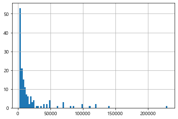
picher['연봉(2018)'].describe()
count       152.000000
mean      18932.236842
std       30940.732924
min        2700.000000
25%        4000.000000
50%        7550.000000
75%       18500.000000
max      230000.000000
Name: 연봉(2018), dtype: float64
picher['연봉(2018)'].hist(bins=100) # 2018년 연봉 분포를 출력
# 5억이상 선수가 많이 없다.
<matplotlib.axes._subplots.AxesSubplot at 0x1267d5c1760>
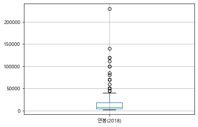
picher.boxplot(column=['연봉(2018)']) # 연봉의 Boxplot을 출력
<matplotlib.axes._subplots.AxesSubplot at 0x1267d56d3d0>
# 회귀분석을 이용할 칼럼
picher_features_df = picher[['승', '패', '세', '홀드', '블론', '경기', '선발', '이닝', '삼진/9',
'볼넷/9', '홈런/9', 'BABIP', 'LOB%', 'ERA', 'RA9-WAR', 'FIP', 'kFIP', 'WAR',
'연봉(2018)', '연봉(2017)']]
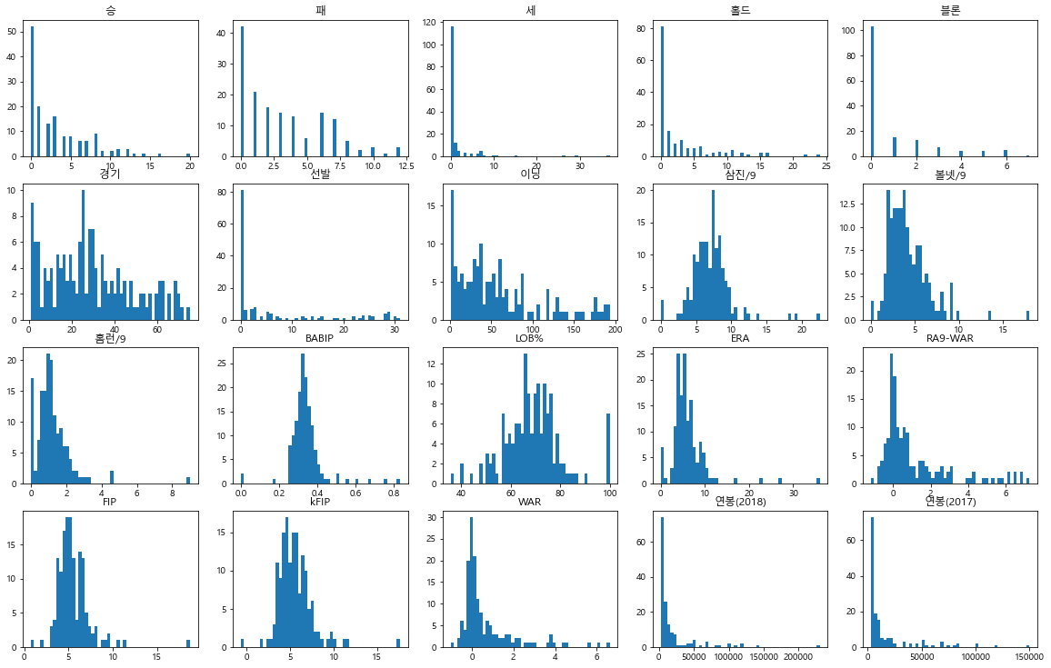
#칼럼마다 그래프 만들기
# 피처 각각에 대한 histogram을 출력
def plot_hist_each_column(df):
    plt.rcParams['figure.figsize'] = [20, 16]
    fig = plt.figure(1)

    # df의 column 갯수 만큼의 subplot을 출력합니다.
    for i in range(len(df.columns)):
        ax = fig.add_subplot(5, 5, i+1) #5 x 5형태로 나타내기
        plt.hist(df[df.columns[i]], bins=50) # 막대 50개
        ax.set_title(df.columns[i])
    plt.show()
plot_hist_each_column(picher_features_df)
연봉예측
#칼럼들의 단위 맞춰주기 : 칼럼 스케일링


# pandas 형태로 정의된 데이터를 출력할 때, scientific-notation이 아닌 float 모양으로 출력
pd.options.mode.chained_assignment = None
# 칼럼 각각에 대한 scaling을 수행하는 함수를 정의
def standard_scaling(df, scale_columns):
    for col in scale_columns:
        series_mean = df[col].mean()
        series_std = df[col].std()
        df[col] = df[col].apply(lambda x: (x-series_mean)/series_std)
    return df
# 칼럼 각각에 대한 scaling을 수행합니다.
scale_columns = ['승', '패', '세', '홀드', '블론', '경기', '선발', '이닝', '삼진/9',
       '볼넷/9', '홈런/9', 'BABIP', 'LOB%', 'ERA', 'RA9-WAR', 'FIP', 'kFIP', 'WAR', '연봉(2017)']
picher_df = standard_scaling(picher, scale_columns)
picher_df = picher_df.rename(columns={'연봉(2018)': 'y'})
picher_df.head(5)
# -5 ~ 5사이로 다 만들어주기
| 선수명 | 팀명 | 승 | 패 | 세 | 홀드 | 블론 | 경기 | 선발 | 이닝 | ... | 홈런/9 | BABIP | LOB% | ERA | RA9-WAR | FIP | kFIP | WAR | y | 연봉(2017) | |
|---|---|---|---|---|---|---|---|---|---|---|---|---|---|---|---|---|---|---|---|---|---|
| 0 | 켈리 | SK | 3.313623 | 1.227145 | -0.306452 | -0.585705 | -0.543592 | 0.059433 | 2.452068 | 2.645175 | ... | -0.442382 | 0.016783 | 0.446615 | -0.587056 | 3.174630 | -0.971030 | -1.058125 | 4.503142 | 140000 | 2.734705 |
| 1 | 소사 | LG | 2.019505 | 2.504721 | -0.098502 | -0.585705 | -0.543592 | 0.059433 | 2.349505 | 2.547755 | ... | -0.668521 | -0.241686 | -0.122764 | -0.519855 | 3.114968 | -1.061888 | -1.073265 | 4.094734 | 120000 | 1.337303 |
| 2 | 양현종 | KIA | 4.348918 | 0.907751 | -0.306452 | -0.585705 | -0.543592 | 0.111056 | 2.554632 | 2.706808 | ... | -0.412886 | -0.095595 | 0.308584 | -0.625456 | 2.973948 | -0.837415 | -0.866361 | 3.761956 | 230000 | 5.329881 |
| 3 | 차우찬 | LG | 1.760682 | 1.227145 | -0.306452 | -0.585705 | -0.543592 | -0.043811 | 2.246942 | 2.350927 | ... | -0.186746 | -0.477680 | 0.558765 | -0.627856 | 2.740722 | -0.698455 | -0.760385 | 2.998081 | 100000 | 3.333592 |
| 4 | 레일리 | 롯데 | 2.537153 | 1.227145 | -0.306452 | -0.585705 | -0.543592 | 0.059433 | 2.452068 | 2.587518 | ... | -0.294900 | -0.196735 | 0.481122 | -0.539055 | 2.751570 | -0.612941 | -0.619085 | 2.809003 | 111000 | 2.734705 |
5 rows × 22 columns
#칼럼들의 단위 맞춰주기 : one-hot-encoding ( 0과1로 표현)

team_encoding = pd.get_dummies(picher_df['팀명'])
picher_df = picher_df.drop('팀명', axis=1)
# axis=1로 행으로쭉
picher_df = picher_df.join(team_encoding)
# 팀칼럼 join
team_encoding.head(5)
| KIA | KT | LG | NC | SK | 두산 | 롯데 | 삼성 | 한화 | |
|---|---|---|---|---|---|---|---|---|---|
| 0 | 0 | 0 | 0 | 0 | 1 | 0 | 0 | 0 | 0 |
| 1 | 0 | 0 | 1 | 0 | 0 | 0 | 0 | 0 | 0 |
| 2 | 1 | 0 | 0 | 0 | 0 | 0 | 0 | 0 | 0 |
| 3 | 0 | 0 | 1 | 0 | 0 | 0 | 0 | 0 | 0 |
| 4 | 0 | 0 | 0 | 0 | 0 | 0 | 1 | 0 | 0 |
picher_df.head()
| 선수명 | 승 | 패 | 세 | 홀드 | 블론 | 경기 | 선발 | 이닝 | 삼진/9 | ... | 연봉(2017) | KIA | KT | LG | NC | SK | 두산 | 롯데 | 삼성 | 한화 | |
|---|---|---|---|---|---|---|---|---|---|---|---|---|---|---|---|---|---|---|---|---|---|
| 0 | 켈리 | 3.313623 | 1.227145 | -0.306452 | -0.585705 | -0.543592 | 0.059433 | 2.452068 | 2.645175 | 0.672099 | ... | 2.734705 | 0 | 0 | 0 | 0 | 1 | 0 | 0 | 0 | 0 |
| 1 | 소사 | 2.019505 | 2.504721 | -0.098502 | -0.585705 | -0.543592 | 0.059433 | 2.349505 | 2.547755 | 0.134531 | ... | 1.337303 | 0 | 0 | 1 | 0 | 0 | 0 | 0 | 0 | 0 |
| 2 | 양현종 | 4.348918 | 0.907751 | -0.306452 | -0.585705 | -0.543592 | 0.111056 | 2.554632 | 2.706808 | 0.109775 | ... | 5.329881 | 1 | 0 | 0 | 0 | 0 | 0 | 0 | 0 | 0 |
| 3 | 차우찬 | 1.760682 | 1.227145 | -0.306452 | -0.585705 | -0.543592 | -0.043811 | 2.246942 | 2.350927 | 0.350266 | ... | 3.333592 | 0 | 0 | 1 | 0 | 0 | 0 | 0 | 0 | 0 |
| 4 | 레일리 | 2.537153 | 1.227145 | -0.306452 | -0.585705 | -0.543592 | 0.059433 | 2.452068 | 2.587518 | 0.155751 | ... | 2.734705 | 0 | 0 | 0 | 0 | 0 | 0 | 1 | 0 | 0 |
5 rows × 30 columns
#회귀 분석을 위한 학습, 테스트 데이터셋 분리
from sklearn import linear_model
from sklearn.model_selection import train_test_split
from sklearn.metrics import mean_squared_error
from math import sqrt

# 학습 데이터와 테스트 데이터로 분리
X = picher_df[picher_df.columns.difference(['선수명', 'y'])]
y = picher_df['y']
X_train, X_test, y_train, y_test = train_test_split(X, y, test_size=0.2, random_state=19)
# 회귀 분석 계수를 학습(회귀 모델 학습)
lr = linear_model.LinearRegression()
model = lr.fit(X_train, y_train)
# 학습된 계수를 출력합니다.
print(lr.coef_)
[ -1481.01733901   -416.68736601 -94136.23649209  -1560.86205158
   1572.00472193   -747.04952389  -1375.53830289   -523.54687556
   3959.10653661    898.37638984  10272.48746451  77672.53804469
  -2434.38947427   -892.11801281    449.91117164   7612.15661812
   1271.04500059  -2810.5564514    5396.97279896  -4797.30275904
   -250.69773139    236.02530053  19130.59021357    854.02604585
   1301.61974637   3613.84063182   -935.07281796  18144.60099745]
picher_df.columns
Index(['선수명', '승', '패', '세', '홀드', '블론', '경기', '선발', '이닝', '삼진/9', '볼넷/9',
       '홈런/9', 'BABIP', 'LOB%', 'ERA', 'RA9-WAR', 'FIP', 'kFIP', 'WAR', 'y',
       '연봉(2017)', 'KIA', 'KT', 'LG', 'NC', 'SK', '두산', '롯데', '삼성', '한화'],
      dtype='object')
예측모델평가
import statsmodels.api as sm

# statsmodel 라이브러리로 회귀 분석을 수행
X_train = sm.add_constant(X_train)
model = sm.OLS(y_train, X_train).fit()
model.summary()
| Dep. Variable: | y | R-squared: | 0.928 |
|---|---|---|---|
| Model: | OLS | Adj. R-squared: | 0.907 |
| Method: | Least Squares | F-statistic: | 44.19 |
| Date: | Tue, 26 Jan 2021 | Prob (F-statistic): | 7.70e-42 |
| Time: | 16:51:12 | Log-Likelihood: | -1247.8 |
| No. Observations: | 121 | AIC: | 2552. |
| Df Residuals: | 93 | BIC: | 2630. |
| Df Model: | 27 | ||
| Covariance Type: | nonrobust |
| coef | std err | t | P>|t| | [0.025 | 0.975] | |
|---|---|---|---|---|---|---|
| const | 1.678e+04 | 697.967 | 24.036 | 0.000 | 1.54e+04 | 1.82e+04 |
| BABIP | -1481.0173 | 1293.397 | -1.145 | 0.255 | -4049.448 | 1087.414 |
| ERA | -416.6874 | 2322.402 | -0.179 | 0.858 | -5028.517 | 4195.143 |
| FIP | -9.414e+04 | 9.43e+04 | -0.998 | 0.321 | -2.81e+05 | 9.31e+04 |
| KIA | 303.1852 | 2222.099 | 0.136 | 0.892 | -4109.462 | 4715.833 |
| KT | 3436.0520 | 2133.084 | 1.611 | 0.111 | -799.831 | 7671.935 |
| LG | 1116.9978 | 2403.317 | 0.465 | 0.643 | -3655.513 | 5889.509 |
| LOB% | -1375.5383 | 1564.806 | -0.879 | 0.382 | -4482.933 | 1731.857 |
| NC | 1340.5004 | 2660.966 | 0.504 | 0.616 | -3943.651 | 6624.652 |
| RA9-WAR | 3959.1065 | 2931.488 | 1.351 | 0.180 | -1862.247 | 9780.460 |
| SK | 2762.4237 | 2243.540 | 1.231 | 0.221 | -1692.803 | 7217.650 |
| WAR | 1.027e+04 | 2532.309 | 4.057 | 0.000 | 5243.823 | 1.53e+04 |
| kFIP | 7.767e+04 | 7.95e+04 | 0.977 | 0.331 | -8.03e+04 | 2.36e+05 |
| 경기 | -2434.3895 | 2953.530 | -0.824 | 0.412 | -8299.515 | 3430.736 |
| 두산 | 971.9293 | 2589.849 | 0.375 | 0.708 | -4170.998 | 6114.857 |
| 롯데 | 2313.9585 | 2566.009 | 0.902 | 0.370 | -2781.627 | 7409.544 |
| 볼넷/9 | 7612.1566 | 6275.338 | 1.213 | 0.228 | -4849.421 | 2.01e+04 |
| 블론 | 1271.0450 | 1242.128 | 1.023 | 0.309 | -1195.576 | 3737.666 |
| 삼성 | -946.5092 | 2482.257 | -0.381 | 0.704 | -5875.780 | 3982.762 |
| 삼진/9 | 5396.9728 | 7286.221 | 0.741 | 0.461 | -9072.019 | 1.99e+04 |
| 선발 | -4797.3028 | 5489.352 | -0.874 | 0.384 | -1.57e+04 | 6103.463 |
| 세 | -250.6977 | 1295.377 | -0.194 | 0.847 | -2823.059 | 2321.663 |
| 승 | 236.0253 | 2215.264 | 0.107 | 0.915 | -4163.049 | 4635.100 |
| 연봉(2017) | 1.913e+04 | 1270.754 | 15.055 | 0.000 | 1.66e+04 | 2.17e+04 |
| 이닝 | 854.0260 | 6623.940 | 0.129 | 0.898 | -1.23e+04 | 1.4e+04 |
| 패 | 1301.6197 | 1935.935 | 0.672 | 0.503 | -2542.763 | 5146.003 |
| 한화 | 5477.8879 | 2184.273 | 2.508 | 0.014 | 1140.355 | 9815.421 |
| 홀드 | -935.0728 | 1637.923 | -0.571 | 0.569 | -4187.663 | 2317.518 |
| 홈런/9 | 1.814e+04 | 1.68e+04 | 1.082 | 0.282 | -1.52e+04 | 5.14e+04 |
| Omnibus: | 28.069 | Durbin-Watson: | 2.025 |
|---|---|---|---|
| Prob(Omnibus): | 0.000 | Jarque-Bera (JB): | 194.274 |
| Skew: | -0.405 | Prob(JB): | 6.52e-43 |
| Kurtosis: | 9.155 | Cond. No. | 3.44e+16 |
Warnings:
[1] Standard Errors assume that the covariance matrix of the errors is correctly specified.
[2] The smallest eigenvalue is 6.73e-31. This might indicate that there are
strong multicollinearity problems or that the design matrix is singular.
# 한글 출력을 위한 사전 설정 단계
mpl.rc('font', family='Malgun Gothic')
plt.rcParams['figure.figsize'] = [20, 16]
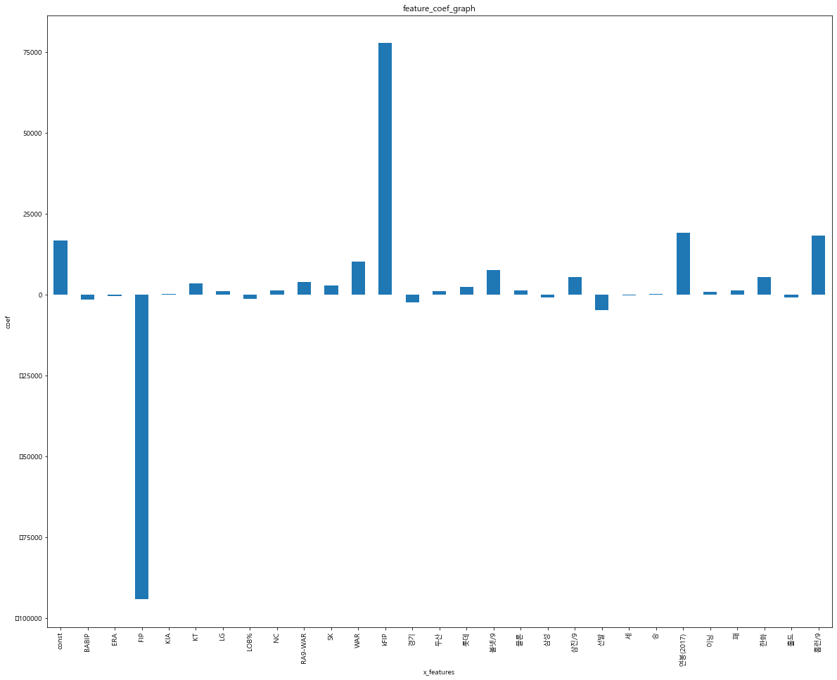
# 회귀 계수를 리스트로 반환
coefs = model.params.tolist()
coefs_series = pd.Series(coefs)
# 변수명을 리스트로 반환
x_labels = model.params.index.tolist()
# 회귀 계수를 출력
ax = coefs_series.plot(kind='bar')
ax.set_title('feature_coef_graph')
ax.set_xlabel('x_features')
ax.set_ylabel('coef')
ax.set_xticklabels(x_labels)
[Text(0, 0, 'const'),
 Text(0, 0, 'BABIP'),
 Text(0, 0, 'ERA'),
 Text(0, 0, 'FIP'),
 Text(0, 0, 'KIA'),
 Text(0, 0, 'KT'),
 Text(0, 0, 'LG'),
 Text(0, 0, 'LOB%'),
 Text(0, 0, 'NC'),
 Text(0, 0, 'RA9-WAR'),
 Text(0, 0, 'SK'),
 Text(0, 0, 'WAR'),
 Text(0, 0, 'kFIP'),
 Text(0, 0, '경기'),
 Text(0, 0, '두산'),
 Text(0, 0, '롯데'),
 Text(0, 0, '볼넷/9'),
 Text(0, 0, '블론'),
 Text(0, 0, '삼성'),
 Text(0, 0, '삼진/9'),
 Text(0, 0, '선발'),
 Text(0, 0, '세'),
 Text(0, 0, '승'),
 Text(0, 0, '연봉(2017)'),
 Text(0, 0, '이닝'),
 Text(0, 0, '패'),
 Text(0, 0, '한화'),
 Text(0, 0, '홀드'),
 Text(0, 0, '홈런/9')]
# 학습 데이터와 테스트 데이터로 분리
X = picher_df[picher_df.columns.difference(['선수명', 'y'])]
y = picher_df['y']
X_train, X_test, y_train, y_test = train_test_split(X, y, test_size=0.2, random_state=19)
# 회귀 분석 모델을 학습
lr = linear_model.LinearRegression()
model = lr.fit(X_train, y_train)
# R2 score
# 회귀 분석 모델을 평가합니다.
print(model.score(X_train, y_train)) # train R2 score를 출력합니다.
print(model.score(X_test, y_test)) # test R2 score를 출력합니다.
0.9276949405576705
0.8860171644977818
# RMSE score
# 회귀 분석 모델을 평가합니다.
y_predictions = lr.predict(X_train)
print(sqrt(mean_squared_error(y_train, y_predictions))) # train RMSE score를 출력합니다.
y_predictions = lr.predict(X_test)
print(sqrt(mean_squared_error(y_test, y_predictions))) # test RMSE score를 출력합니다.
7282.718684746374
14310.69643688913
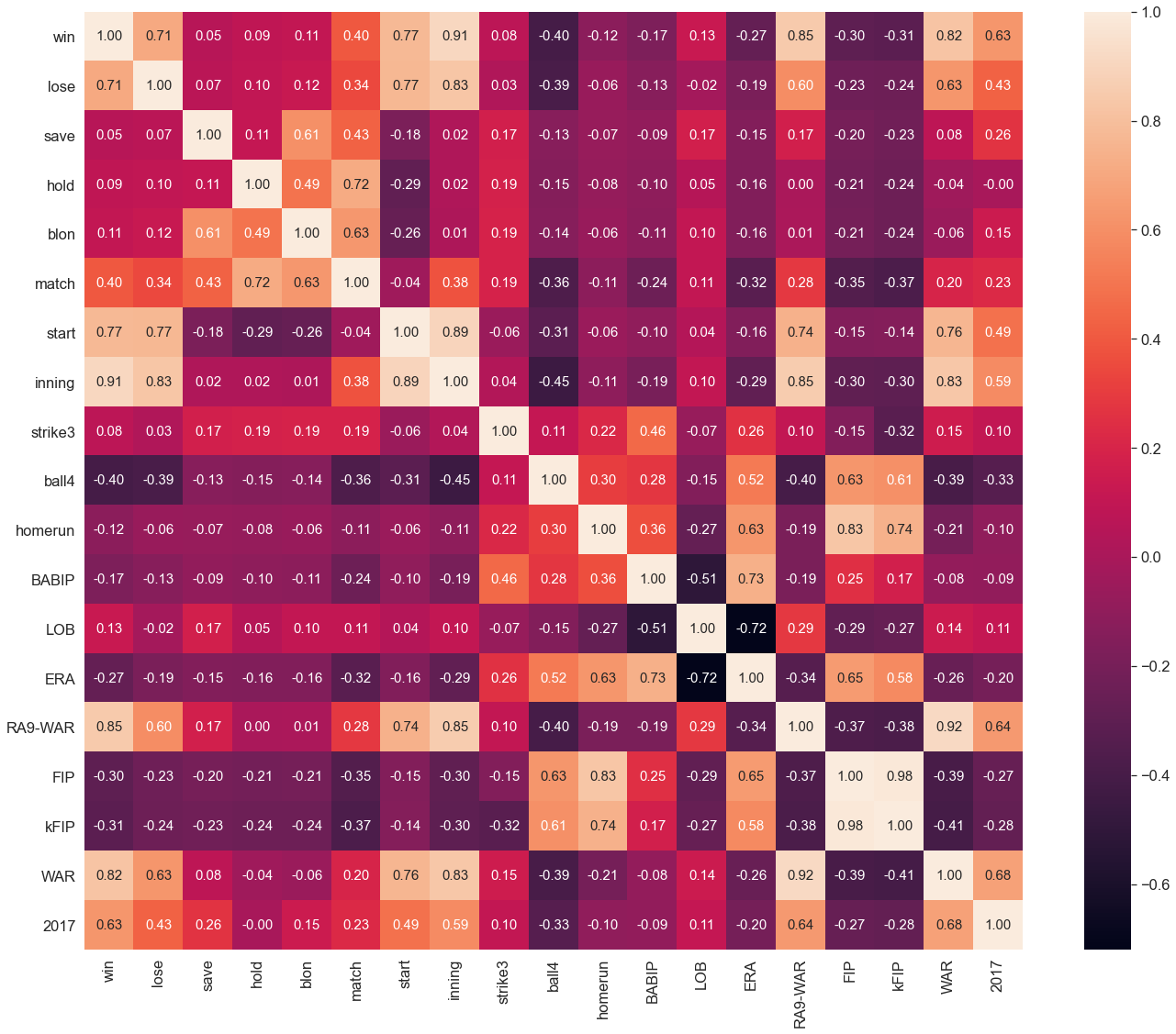
칼럼들의 상관관계
import seaborn as sns

# 칼럼간의 상관계수 행렬을 계산
corr = picher_df[scale_columns].corr(method='pearson')
show_cols = ['win', 'lose', 'save', 'hold', 'blon', 'match', 'start',
             'inning', 'strike3', 'ball4', 'homerun', 'BABIP', 'LOB',
             'ERA', 'RA9-WAR', 'FIP', 'kFIP', 'WAR', '2017']

# corr 행렬 히트맵을 시각화
plt.rc('font', family='Malgun Gothic')
sns.set(font_scale=1.5)
hm = sns.heatmap(corr.values,
            cbar=True,
            annot=True,
            square=True,
            fmt='.2f',
            annot_kws={'size': 15},
            yticklabels=show_cols,
            xticklabels=show_cols)

plt.tight_layout()
plt.show()
회귀분석 예측 성능을 높이기 위한 방법 : 다중공선성 확인
from statsmodels.stats.outliers_influence import variance_inflation_factor

# 칼럼마다의 VIF 계수를 출력합니다.
vif = pd.DataFrame()
vif["VIF Factor"] = [variance_inflation_factor(X.values, i) for i in range(X.shape[1])]
vif["features"] = X.columns
vif.round(1)
| VIF Factor | features | |
|---|---|---|
| 0 | 3.2 | BABIP |
| 1 | 10.6 | ERA |
| 2 | 14238.3 | FIP |
| 3 | 1.1 | KIA |
| 4 | 1.1 | KT |
| 5 | 1.1 | LG |
| 6 | 4.3 | LOB% |
| 7 | 1.1 | NC |
| 8 | 13.6 | RA9-WAR |
| 9 | 1.1 | SK |
| 10 | 10.4 | WAR |
| 11 | 10264.1 | kFIP |
| 12 | 14.6 | 경기 |
| 13 | 1.2 | 두산 |
| 14 | 1.1 | 롯데 |
| 15 | 57.8 | 볼넷/9 |
| 16 | 3.0 | 블론 |
| 17 | 1.2 | 삼성 |
| 18 | 89.5 | 삼진/9 |
| 19 | 39.6 | 선발 |
| 20 | 3.1 | 세 |
| 21 | 8.0 | 승 |
| 22 | 2.5 | 연봉(2017) |
| 23 | 63.8 | 이닝 |
| 24 | 5.9 | 패 |
| 25 | 1.1 | 한화 |
| 26 | 3.8 | 홀드 |
| 27 | 425.6 | 홈런/9 |
# 적절한 칼럼으로 다시 학습하기
# 칼럼을 재선정합니다.
X = picher_df[['FIP', 'WAR', '볼넷/9', '삼진/9', '연봉(2017)']]
y = picher_df['y']
X_train, X_test, y_train, y_test = train_test_split(X, y, test_size=0.2, random_state=19)
# 모델을 학습
lr = linear_model.LinearRegression()
model = lr.fit(X_train, y_train)
# 결과를 출력
print(model.score(X_train, y_train)) # train R2 score를 출력
print(model.score(X_test, y_test)) # test R2 score를 출력
0.9150591192570362
0.9038759653889864
# 회귀 분석 모델을 평가
y_predictions = lr.predict(X_train)
print(sqrt(mean_squared_error(y_train, y_predictions))) # train RMSE score를 출력
y_predictions = lr.predict(X_test)
print(sqrt(mean_squared_error(y_test, y_predictions))) # test RMSE score를 출력
7893.462873347692
13141.866063591087
# 칼럼마다의 VIF 계수를 출력합니다.
X = picher_df[['FIP', 'WAR', '볼넷/9', '삼진/9', '연봉(2017)']]
vif = pd.DataFrame()
vif["VIF Factor"] = [variance_inflation_factor(X.values, i) for i in range(X.shape[1])]
vif["features"] = X.columns
vif.round(1)
| VIF Factor | features | |
|---|---|---|
| 0 | 1.9 | FIP |
| 1 | 2.1 | WAR |
| 2 | 1.9 | 볼넷/9 |
| 3 | 1.1 | 삼진/9 |
| 4 | 1.9 | 연봉(2017) |
분석결과 시각화
# 2018년 연봉을 예측하여 데이터프레임의 column으로 생성
X = picher_df[['FIP', 'WAR', '볼넷/9', '삼진/9', '연봉(2017)']]
predict_2018_salary = lr.predict(X)
picher_df['예측연봉(2018)'] = pd.Series(predict_2018_salary)
# 원래의 데이터 프레임을 다시 로드
picher = pd.read_csv(picher_file_path)
picher = picher[['선수명', '연봉(2017)']]

# 원래의 데이터 프레임에 2018년 연봉 정보를 합치기
result_df = picher_df.sort_values(by=['y'], ascending=False)
result_df.drop(['연봉(2017)'], axis=1, inplace=True, errors='ignore')
result_df = result_df.merge(picher, on=['선수명'], how='left')
result_df = result_df[['선수명', 'y', '예측연봉(2018)', '연봉(2017)']]
result_df.columns = ['선수명', '실제연봉(2018)', '예측연봉(2018)', '작년연봉(2017)']

# 재계약하여 연봉이 변화한 선수만을 대상으로 관찰
result_df = result_df[result_df['작년연봉(2017)'] != result_df['실제연봉(2018)']]
result_df = result_df.reset_index()
result_df = result_df.iloc[:10, :]
result_df.head(10)
| index | 선수명 | 실제연봉(2018) | 예측연봉(2018) | 작년연봉(2017) | |
|---|---|---|---|---|---|
| 0 | 0 | 양현종 | 230000 | 163930.148696 | 150000 |
| 1 | 1 | 켈리 | 140000 | 120122.822204 | 85000 |
| 2 | 2 | 소사 | 120000 | 88127.019455 | 50000 |
| 3 | 4 | 레일리 | 111000 | 102253.697589 | 85000 |
| 4 | 7 | 피어밴드 | 85000 | 58975.725734 | 35000 |
| 5 | 13 | 배영수 | 50000 | 56873.662417 | 55000 |
| 6 | 21 | 안영명 | 35000 | 22420.790838 | 20000 |
| 7 | 22 | 채병용 | 30000 | 21178.955105 | 25000 |
| 8 | 23 | 류제국 | 29000 | 45122.360087 | 35000 |
| 9 | 24 | 박정진 | 25000 | 29060.748299 | 33000 |
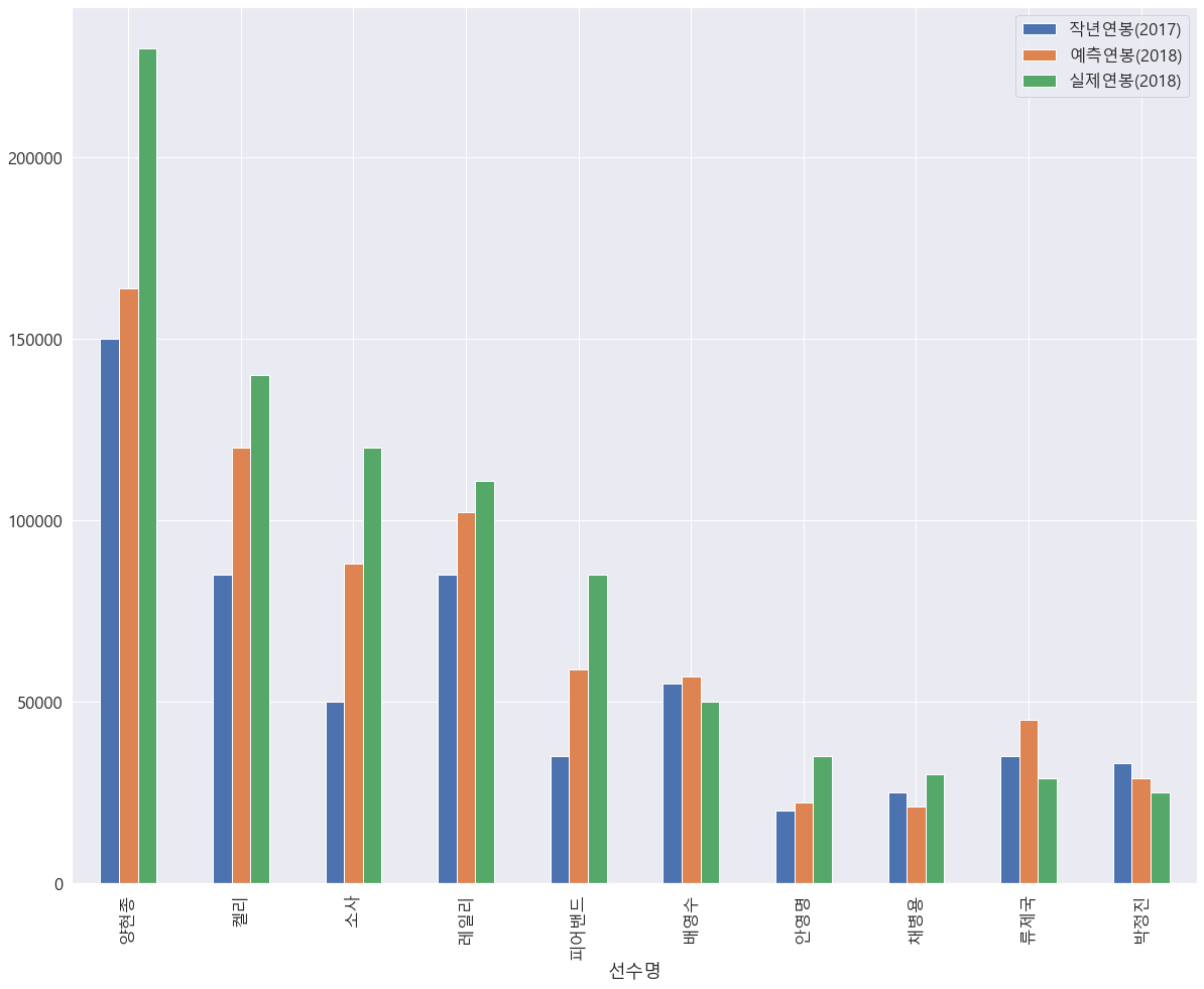
# 선수별 연봉 정보(작년 연봉, 예측 연봉, 실제 연봉)를 bar 그래프로 출력
mpl.rc('font', family='Malgun Gothic')
result_df.plot(x='선수명', y=['작년연봉(2017)', '예측연봉(2018)', '실제연봉(2018)'], kind="bar")
<matplotlib.axes._subplots.AxesSubplot at 0x1267d895f70>