비트코인시세예측
in Study on datavisualization
비트코인 시세 예측하기
# -*- coding: utf-8 -*-

%matplotlib inline

import pandas as pd
import numpy as np
import matplotlib.pyplot as plt

import warnings
warnings.filterwarnings("ignore")
# Data Source : https://www.blockchain.com/ko/charts/market-price?timespan=60days

file_path = 'data/market-price.csv'
bitcoin_df = pd.read_csv(file_path, names = ['day', 'price'])
# 기본 정보를 출력
print(bitcoin_df.shape)
print(bitcoin_df.info())
#칼럼은 날짜와가격
(365, 2)
<class 'pandas.core.frame.DataFrame'>
RangeIndex: 365 entries, 0 to 364
Data columns (total 2 columns):
 #   Column  Non-Null Count  Dtype
---  ------  --------------  -----
 0   day     365 non-null    object
 1   price   365 non-null    float64
dtypes: float64(1), object(1)
memory usage: 5.8+ KB
None
bitcoin_df.tail()
| day | price | |
|---|---|---|
| 360 | 2018-08-22 00:00:00 | 6575.229167 |
| 361 | 2018-08-23 00:00:00 | 6434.881667 |
| 362 | 2018-08-24 00:00:00 | 6543.645714 |
| 363 | 2018-08-25 00:00:00 | 6719.429231 |
| 364 | 2018-08-26 00:00:00 | 6673.274167 |
# to_datetime으로 day 피처를 시계열 칼럼으로 변환
bitcoin_df['day'] = pd.to_datetime(bitcoin_df['day'])

# day 데이터프레임의 index로 설정 (시각화 하기 쉽다)
bitcoin_df.index = bitcoin_df['day']
bitcoin_df.set_index('day', inplace=True)
bitcoin_df.head()
| price | |
|---|---|
| day | |
| 2017-08-27 | 4354.308333 |
| 2017-08-28 | 4391.673517 |
| 2017-08-29 | 4607.985450 |
| 2017-08-30 | 4594.987850 |
| 2017-08-31 | 4748.255000 |
bitcoin_df.describe()
| price | |
|---|---|
| count | 365.000000 |
| mean | 8395.863578 |
| std | 3239.804756 |
| min | 3319.630000 |
| 25% | 6396.772500 |
| 50% | 7685.633333 |
| 75% | 9630.136277 |
| max | 19498.683333 |
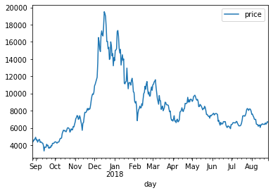
# 일자별 비트코인 시세를 시각화
bitcoin_df.plot()
plt.show()
ARIMA를 활용한 시세 예측
# ARIMA 모델 활용하기

from statsmodels.tsa.arima_model import ARIMA
import statsmodels.api as sm

# (AR=2, 차분=1, MA=2) 파라미터로 ARIMA 모델을 학습
model = ARIMA(bitcoin_df.price.values, order=(2,1,2))
model_fit = model.fit(trend='c', full_output=True, disp=True)
print(model_fit.summary())
                             ARIMA Model Results
==============================================================================
Dep. Variable:                    D.y   No. Observations:                  364
Model:                 ARIMA(2, 1, 2)   Log Likelihood               -2787.553
Method:                       css-mle   S.D. of innovations            512.415
Date:                Tue, 26 Jan 2021   AIC                           5587.107
Time:                        17:18:43   BIC                           5610.490
Sample:                             1   HQIC                          5596.400

==============================================================================
                 coef    std err          z      P>|z|      [0.025      0.975]
------------------------------------------------------------------------------
const          6.1416     27.794      0.221      0.825     -48.334      60.618
ar.L1.D.y     -0.3790      1.829     -0.207      0.836      -3.964       3.206
ar.L2.D.y      0.1585      1.192      0.133      0.894      -2.178       2.495
ma.L1.D.y      0.4571      1.825      0.250      0.802      -3.120       4.034
ma.L2.D.y     -0.1940      1.339     -0.145      0.885      -2.819       2.431
                                    Roots
=============================================================================
                  Real          Imaginary           Modulus         Frequency
-----------------------------------------------------------------------------
AR.1           -1.5864           +0.0000j            1.5864            0.5000
AR.2            3.9777           +0.0000j            3.9777            0.0000
MA.1           -1.3797           +0.0000j            1.3797            0.5000
MA.2            3.7354           +0.0000j            3.7354            0.0000
-----------------------------------------------------------------------------
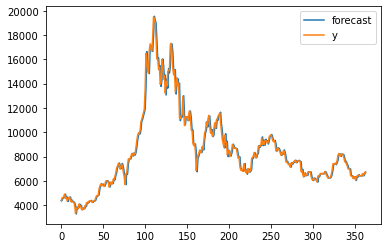
# 모델의 성능 & 예측 결과 시각화
fig = model_fit.plot_predict() # 학습 데이터에 대한 예측 결과 (첫번째 그래프)
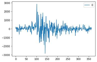
residuals = pd.DataFrame(model_fit.resid) # 잔차의 변동을 시각화 (두번째 그래프)
residuals.plot()
<matplotlib.axes._subplots.AxesSubplot at 0x26e2442b190>
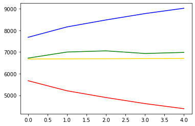
예측 결과인 마지막 5일의 예측값을 실제 데이터와 비교
# 예측 결과인 마지막 5일의 예측값을 실제 데이터와 비교

forecast_data = model_fit.forecast(steps=5) # 학습 데이터셋으로부터 5일 뒤를 예측

# 테스트 데이터셋을 불러옵니다.
test_file_path = 'data/market-price-test.csv' # 실제데이터
bitcoin_test_df = pd.read_csv(test_file_path, names=['ds', 'y'])

pred_y = forecast_data[0].tolist() # 마지막 5일의 예측 데이터입니다. (2018-08-27 ~ 2018-08-31)
test_y = bitcoin_test_df.y.values # 실제 5일 가격 데이터입니다. (2018-08-27 ~ 2018-08-31)
pred_y_lower = [] # 마지막 5일의 예측 데이터의 최소값입니다.
pred_y_upper = [] # 마지막 5일의 예측 데이터의 최대값입니다.
for lower_upper in forecast_data[2]:
    lower = lower_upper[0]
    upper = lower_upper[1]
    pred_y_lower.append(lower)
    pred_y_upper.append(upper)
plt.plot(pred_y, color="gold") # 모델이 예상한 가격 그래프
plt.plot(pred_y_lower, color="red") # 모델이 예상한 최소가격 그래프
plt.plot(pred_y_upper, color="blue") # 모델이 예상한 최대가격 그래프
plt.plot(test_y, color="green") # 실제 가격 그래프
[<matplotlib.lines.Line2D at 0x26e244dc3d0>]
plt.plot(pred_y, color="gold") # 모델이 예상한 가격 그래프
plt.plot(test_y, color="green") # 실제 가격 그래프
[<matplotlib.lines.Line2D at 0x26e24534910>]
from sklearn.metrics import mean_squared_error, r2_score
from math import sqrt

rmse = sqrt(mean_squared_error(pred_y, test_y))
print(rmse)
#test RMSE 점수 : 271.38881165460765
271.38881165460765
Facebook Prophet 활용하기
from fbprophet import Prophet
Importing plotly failed. Interactive plots will not work.
# prophet을 사용하기 위해서는 다음과 같이 피처의 이름을 변경해야  : 'ds', 'y'
bitcoin_df = pd.read_csv(file_path, names=['ds', 'y'])
prophet = Prophet(seasonality_mode='multiplicative',
                  yearly_seasonality=True,
                  weekly_seasonality=True, daily_seasonality=True,
                  changepoint_prior_scale=0.5)
prophet.fit(bitcoin_df)
<fbprophet.forecaster.Prophet at 0x26e283e0b80>
# 5일을 내다보며 예측
future_data = prophet.make_future_dataframe(periods=5, freq='d')
forecast_data = prophet.predict(future_data)
forecast_data.tail(5)
| ds | trend | yhat_lower | yhat_upper | trend_lower | trend_upper | daily | daily_lower | daily_upper | multiplicative_terms | ... | weekly | weekly_lower | weekly_upper | yearly | yearly_lower | yearly_upper | additive_terms | additive_terms_lower | additive_terms_upper | yhat | |
|---|---|---|---|---|---|---|---|---|---|---|---|---|---|---|---|---|---|---|---|---|---|
| 365 | 2018-08-27 | 738.543896 | 6226.354661 | 7523.184197 | 738.543896 | 738.543896 | 9.563964 | 9.563964 | 9.563964 | 8.374726 | ... | -0.006602 | -0.006602 | -0.006602 | -1.182636 | -1.182636 | -1.182636 | 0.0 | 0.0 | 0.0 | 6923.647020 |
| 366 | 2018-08-28 | 742.612648 | 6331.158178 | 7684.153133 | 742.612648 | 742.612648 | 9.563964 | 9.563964 | 9.563964 | 8.452304 | ... | 0.019974 | 0.019974 | 0.019974 | -1.131634 | -1.131634 | -1.131634 | 0.0 | 0.0 | 0.0 | 7019.400574 |
| 367 | 2018-08-29 | 746.681400 | 6309.449564 | 7769.245266 | 745.975687 | 746.681400 | 9.563964 | 9.563964 | 9.563964 | 8.421478 | ... | -0.046634 | -0.046634 | -0.046634 | -1.095851 | -1.095851 | -1.095851 | 0.0 | 0.0 | 0.0 | 7034.842537 |
| 368 | 2018-08-30 | 750.750152 | 6359.511516 | 7822.480347 | 742.394998 | 752.714854 | 9.563964 | 9.563964 | 9.563964 | 8.468117 | ... | -0.017649 | -0.017649 | -0.017649 | -1.078198 | -1.078198 | -1.078198 | 0.0 | 0.0 | 0.0 | 7108.190099 |
| 369 | 2018-08-31 | 754.818904 | 6392.727069 | 7958.671178 | 738.744214 | 768.244440 | 9.563964 | 9.563964 | 9.563964 | 8.518827 | ... | 0.035872 | 0.035872 | 0.035872 | -1.081008 | -1.081008 | -1.081008 | 0.0 | 0.0 | 0.0 | 7184.990775 |
5 rows × 22 columns
forecast_data[['ds', 'yhat', 'yhat_lower', 'yhat_upper']].tail(5)
| ds | yhat | yhat_lower | yhat_upper | |
|---|---|---|---|---|
| 365 | 2018-08-27 | 6923.647020 | 6226.354661 | 7523.184197 |
| 366 | 2018-08-28 | 7019.400574 | 6331.158178 | 7684.153133 |
| 367 | 2018-08-29 | 7034.842537 | 6309.449564 | 7769.245266 |
| 368 | 2018-08-30 | 7108.190099 | 6359.511516 | 7822.480347 |
| 369 | 2018-08-31 | 7184.990775 | 6392.727069 | 7958.671178 |
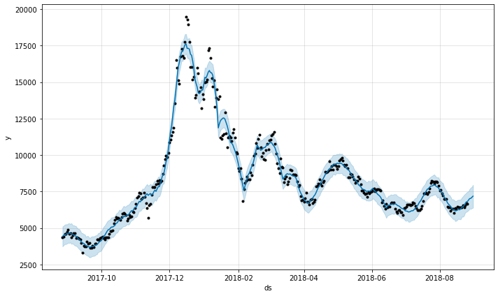
#전체 데이터를 기반으로 학습한, 5일 단위의 예측 결과를 시각화
fig1 = prophet.plot(forecast_data)
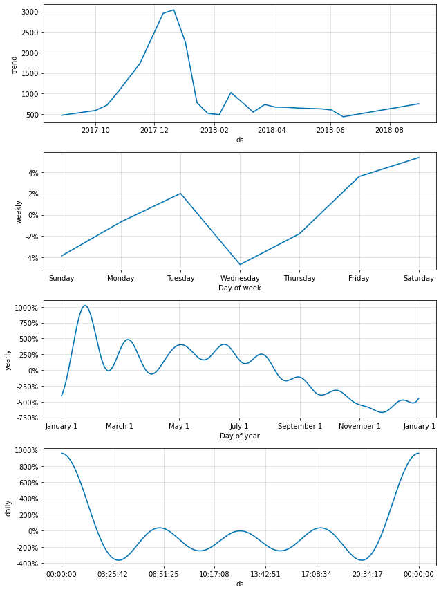
# seasonality_mode로 설정했었던 기간별 트렌드 정보를 시각화
fig2 = prophet.plot_components(forecast_data)
실제 데이터와의 비교
bitcoin_test_df = pd.read_csv(test_file_path, names=['ds', 'y'])

pred_y = forecast_data.yhat.values[-5:] # 마지막 5일의 예측 데이터입니다. (2018-08-27 ~ 2018-08-31)
test_y = bitcoin_test_df.y.values # 실제 5일 가격 데이터입니다. (2018-08-27 ~ 2018-08-31)
pred_y_lower = forecast_data.yhat_lower.values[-5:] # 마지막 5일의 예측 데이터의 최소값
pred_y_upper = forecast_data.yhat_upper.values[-5:] # 마지막 5일의 예측 데이터의 최대값
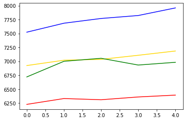
plt.plot(pred_y, color="gold") # 모델이 예상한 가격 그래프
plt.plot(pred_y_lower, color="red") # 모델이 예상한 최소가격 그래프
plt.plot(pred_y_upper, color="blue") # 모델이 예상한 최대가격 그래프
plt.plot(test_y, color="green") # 실제 가격 그래프
[<matplotlib.lines.Line2D at 0x26e2ae87be0>]
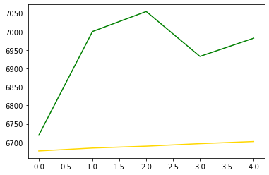
plt.plot(pred_y, color="gold") # 모델이 예상한 가격 그래프
plt.plot(test_y, color="green") # 실제 가격 그래프
[<matplotlib.lines.Line2D at 0x26e2ae51940>]
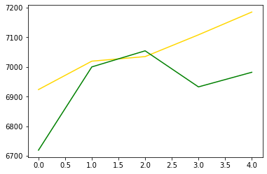
rmse = sqrt(mean_squared_error(pred_y, test_y))
print(rmse)
# test RMSE 점수 : 151.367832019998
151.367832019998